AI-Based Predictive System for Sold Liters of Gasoline

TL;DR: Developed a Jupyter notebook to predict gasoline sales, deployed the best model with Docker using BentoML in Azure, retrained daily to avoid drift. Built a simulator to test how many liters of gasoline will be sold depending on several factors.
The project is about developing a system that:
- Analyse the gas station sales data, including prices, holidays and weather.
- Observes wether competitors are <<copying>> the prices.
- Predicts the amount of gasoline that will be sold in the next
Xhours. - Deploys the best model with Docker using BentoML in Azure.
- Retrains the model daily to avoid drift.
- Build a simulator to test how many liters of gasoline will be sold depending on several factors.
Every analysis made is done using Jupyter Notebooks and a conda environment, to keep the dependencies in check. Time series data is analysed and we will apply the proper techniques to handle it.
Technologies
Analysis of the Data
Data is collected privately from the gas station and it cannot be shared. Prices, holidays, weather, competitor prices and others are considered because they affect the sales. Sold liters of gasoline is a type of time series data that follows a relatively predictable pattern, but it is also very noisy. Sometimes, a trailer truck can come and buy 300 liters and the next day, it will only be some cars or motorcycles, which can fill up different amounts of gasoline.

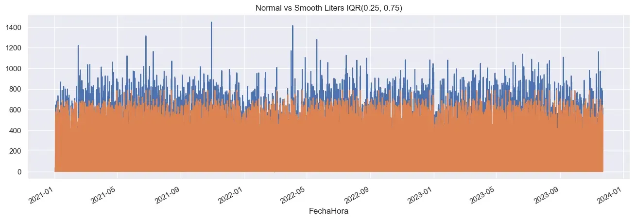
Noisy data presents a significant challenge for prediction because, while it is not entirely random, it relies on variables that are difficult to measure, such as individual consumer needs, economic conditions, and even customer emotions. Our predictive models perform better when we reduce the noise in the data. To achieve this while preserving as much valuable information as possible, we employed:
- IQR to remove the outliers. In this case,
- Accumulated sum of the sold liters to smooth the data without loosing information.
The further analysis includes a variety of visualizations to explore and understand the data in depth. These visualizations consist of histograms to examine the distribution of variables, heatmaps showing correlations using both Spearman and Pearson methods, and boxplots to identify outliers within the variables. Additionally, the analysis focuses on the sold liters time series, including boxplots of sold liters segmented by season, month, week, day, and hour. Moreover, it includes plots of the average sold liters per weekday, supplemented with ±1 standard deviation to provide insights into the variability.
Time Series Analysis
To analyse the sold liters time series, we need to see:
- Stationarity. The data is stationary if the mean and variance are constant over time. We can use the Augmented Dickey-Fuller test to check it.
- Seasonality. The data has a seasonal component if it repeats over time. We can use the autocorrelation function to check it.
- Trend. The data has a trend if it increases or decreases over time. We can use the rolling mean and rolling standard deviation to check it.
The time series is stationary, which means that the mean and variance are constant over time. The autocorrelation plot shows that there is a short-term memory effect at the first lag and a long-term memory effect at the 24th lag. The partial autocorrelation plot shows that there is a long-term memory effect at the 24th lag, which decays over the time, meaning that recent data has more influence than older data.
Competitors prices analysis
To complete the analysis, we need to know if competitors are copying the prices. In this case, using a correlation chart is useless, becase all prices are follow the oil prices which they all buy, so correlation is over 98%. We can use:
- Cross-correlation. To see if the prices of the competitors are correlated with the prices of the gas station.
- Granger Causality. To see if the prices of the competitors are granger causing the prices of the gas station. this does not mean causality but wether a time series can be forecasted using another time series.
- Impulse-Response Function. It show how the prices of the competitors affect the prices of the gas station when there is a shock of 1 standard deviation in the prices of the target gas station.
The cross-correlation plot did not throw any significate correlation between the prices of the competitors and the prices of the target gas station. The Granger Causality test did throw some significate results in some lags. To confirm the results, we used the Impulse-Response Function, to show if a shock in the prices of the target gas station affects the prices of the competitors. It showed that one competitor seemed to be affected by the prices of the target gas station. To clear the doubts, we used an ARIMA model to forecast the prices of that competitor using the prices of the target gas station.
We cannot say that any competitor is copying the prices of the target gas station with certainty, but we can say that one competitor is affected by the prices of the target gas station and can be forecasted using the prices of the target gas station, even though prices are very similar.
Predictive Model
To predict the sold liters of gasoline, we need to choose a model that can handle time series data. First, we need to create derived variables that can help, preprocess the data and choose the best model. After that, we need to optimize the hyperparameters of the best model to get the best results.
Data Preprocessing
In production, data is collected with a delay of 24 hours. As we saw in the partial autocorrelation plot, the 24th lag is the most important, so we still have margin the make good predictions. So, we need to:
- Drop NaN values. As we have a lot of data, we can drop the NaN values.
- Shift data 24 hours. To train the model with the data that we will have in production.
- Smooth data. Using IQR and the accumulated sum of the sold liters as we saw before.
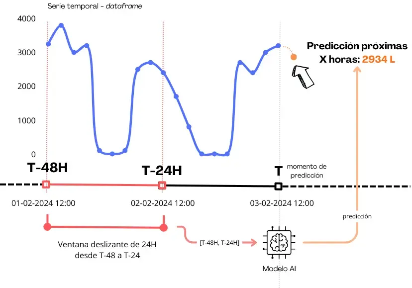
- Create sliding windows. As we saw in the partial autocorrelation plot, the influence of the data decays over time, so we need to create sliding windows to capture the most recent data, avoiding old trends and keeping the most recent ones.
- Split data. We need to split the data into training and testing data.
- Reshape and Normalize data. We need to reshape the data to fit the model and normalize it to avoid the model to be biased by the scale of the data.

The sliding window showed that the best window size is 24 hours, which is the same as the delay of the data. Window of more than 24 hours did not improve the model, but a window of less than 24 hours did not capture sufficient data. The following code provides the function used to create the sliding window:
def split_sequence(sequence, n_steps_in, n_steps_out):
    X, y = list(), list()
    for i in range(len(sequence)):
        # find the end of this pattern
        end_ix = i + n_steps_in
        out_end_ix = end_ix + n_steps_out
        if out_end_ix > len(sequence):
            break
        seq_x, seq_y = sequence[i:end_ix][:,:-1], sequence[end_ix-1:out_end_ix-1, -1]
        X.append(seq_x)
        y.append(seq_y)
    return np.array(X), np.array(y)
Model Selection
We need to choose a model that can handle time series data. We tested several models with a sliding window of 24H, such as:
- ARIMA. It is a simple model that can handle time series data. As we did plot the autocorrelation and partial autocorrelation plots, we know that the data is stationary and has a seasonal component, so ARIMA is a good model to start with.
- XGBoost. It is a more complex model that can handle time series data. Captures non-linear relationships and complex patterns in the data.
- LSTM. It is a model that can handle time series data. It is a good model to use when we have a lot of data and we have a lot of features, capturing short-term and long-term memory effects. It also captures complex pattern but training is slower than XGBoost.
The LSTM model was overfitting the data, so we chose the XGBoost model. Also,the XGBoost model is faster to train than the LSTM model. We tested the models using the sliding window and the best model was XGBoost. Results showed that the models capture the seasonaty and trend successfully, but noise was ignored and the models did not highest and lowest values, even using IQR smoothing.
We also analysed residuals of the models to see if there was any pattern in the data that the model did not capture. The residuals QQ-plot showed that the residuals were normally distributed in most cases, and the residuals line plot over the time showed that the residuals were distributed quite randomly, meaning that the model captured the data quite well.
Model optimization
In this case, once our model is chosen, we need to optimize it to get the best results. We used Optuna library to optimize
the hyperparameters of the XGBoost model. The model improved slightly, but it is better than nothing.
Deployment
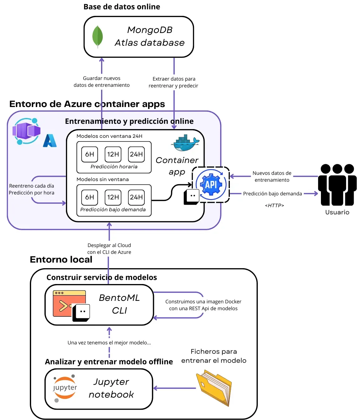
After choosing the best model, we deployed it using Docker and BentoML in Azure. The process is simple, we just need to
use the bentoml build && bentoml containerize --opt platform=linux/amd64 liters_service:latest command to build the Docker
image and then push it to the Azure Container Registry. We can use the Azure CLI to deploy the container to the Azure Container
Registry. After that, we can use the Azure CLI to deploy that container as an Azure Container App.

As we can see in Figure 3, we deployed 2 types of models: with and without sliding windows. The model with sliding windows is used to make hourly predictions and the model without sliding windows is used to make on demand predictions. Last one has no sliding windows because
Every type of model has 3 models: one for every range of hours we want to predict —6, 12 and 24 hours—. The models are retrained daily to avoid data drift, which is a common problem in time series data and can make the model to make bad predictions.
Simulator
To test the model, we built a simulator that can simulate the amount of gasoline that will be sold depending on the sale price, the competitor prices and the day. We can make a REST API call to the Azure Container App to get the predictions by tweaking these variables, achieving a simulation approximation. It is not perfect, an the model will not now what to do when unseen values are passed.
Conclusion
We developed a system that can predict the amount of gasoline that will be sold in the next X hours. The system is deployed
in Azure and retrained daily to avoid drift. We also built a simulator to test how many liters of gasoline will be sold
depending on the sale price, competitor prices and the day. The system is not perfect, but it is a good start to make better
predictions and improve the sales of the gas station.